Building a Product Recommender at Scale

Overview

I set out to figure out which products to suggest to each shopper so they keep finding things they actually want.

• E-commerce growth makes personalized recommendations a core driver of engagement, conversion, and repeat purchases.
• Goal: predict how a user would rate an unseen item and surface the top items most likely to be relevant to them.
• I treat relevance with a threshold rating of 7 (on a 1-10 scale) to score recommendations as relevant or not.
• I compare four recommender families to see which best balances accuracy and useful top-N ranking.
• Success is measured by RMSE on held-out ratings plus precision@k and recall@k for the recommended lists.

Methodology

flowchart LR
  A["User-Item Ratings"] --> B[EDA & Filtering]
  B --> C["Approaches: Popularity / Collaborative Filtering / SVD"]
  C --> D["Evaluate: RMSE / Precision@K"]
  D --> E[Top-N Recommendations]

The Data

I started with over a million product ratings and cleaned them down to the ones that actually carry signal.

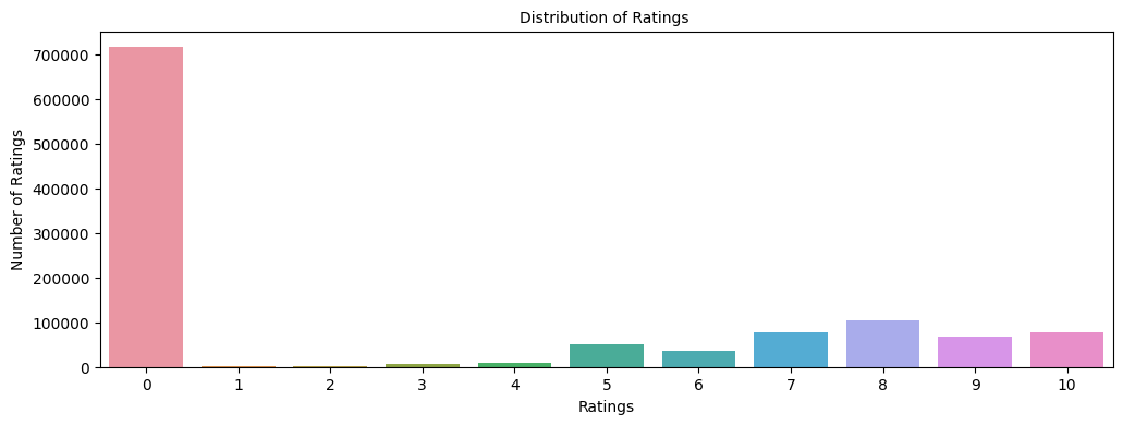
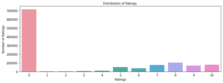
• Raw ratings data held 1,149,780 observations across 7 columns, merged from the ratings and item tables.
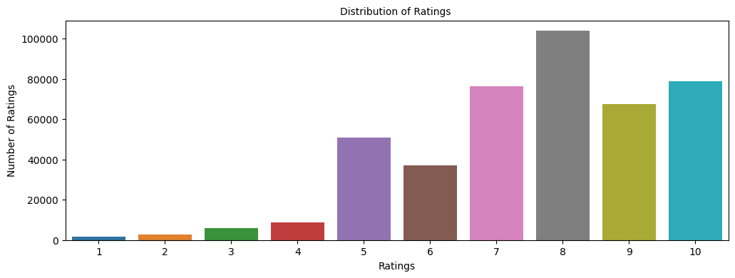
• Ratings of 0 dominated (~700K) and represent missing values, so I dropped them, leaving 433,671 real ratings.
• The cleaned set spans 77,805 unique users and 185,973 unique items on a 1-10 explicit rating scale.
• A full user-item matrix would hold ~14.5 billion cells, so the data is extremely sparse with one rating per user-item pair.
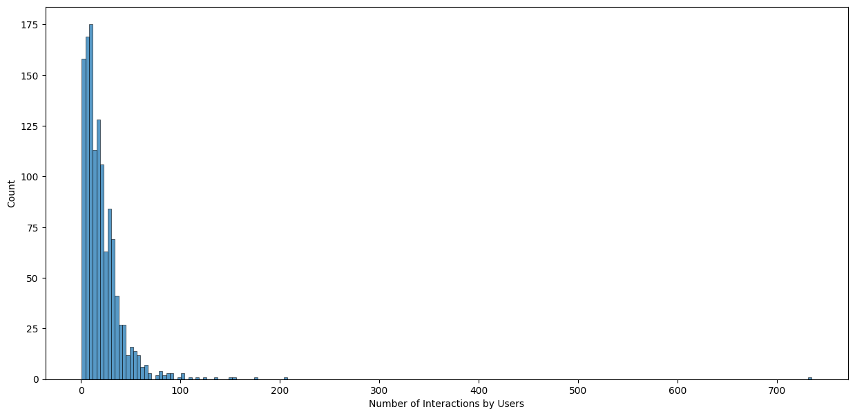
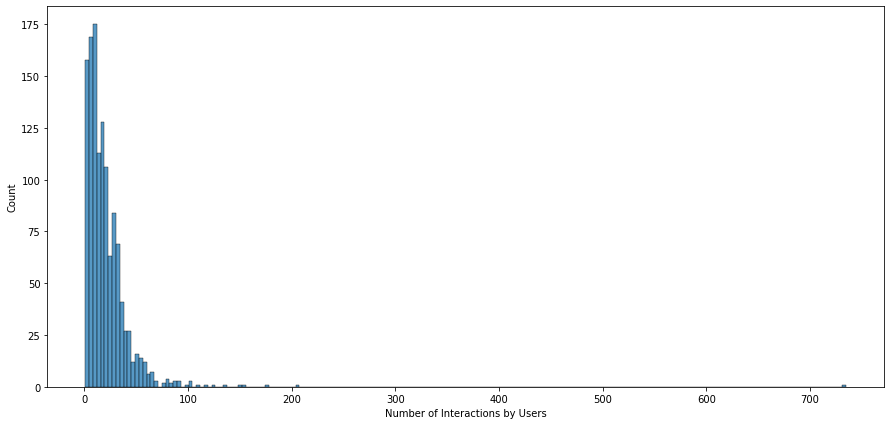
• The most-rated item drew 707 ratings and the most active user rated 8,524 items, showing a long-tail of activity.

Exploratory Analysis

I looked at how ratings and activity are spread out before deciding how to model them.

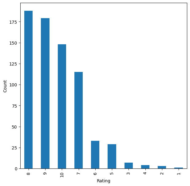
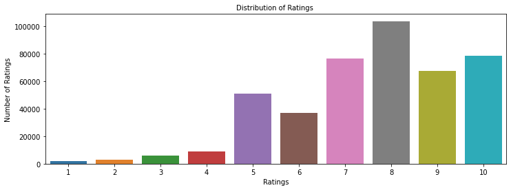
• After removing zeros, rating 8 is most common (~100K), followed by 10 and 7 (~80K each); 1-4 are rare.
• This positive skew means relevance (>=7) is common, which shapes how precision and recall behave.
• The user-item interaction distribution is heavily right-skewed: few items get many ratings, most get very few.
• To make modeling tractable I filtered to active users and well-rated items rather than the full sparse matrix.
• These patterns motivate a popularity baseline plus personalized collaborative filtering on the dense core.

Recommender Approaches

I built four kinds of recommender, from a simple popularity ranking to a learned matrix-factorization model.

• Model 1 - Rank-based: ranks items by average rating with a minimum-interaction threshold, solving cold start.
• Model 2 - User-user collaborative filtering with KNNBasic and cosine similarity over shared ratings.
• Model 3 - Item-item collaborative filtering, computing similarity between items instead of users.
• Model 4 - Matrix factorization with SVD, learning latent user and item factors via regularized SGD.
• I tuned each model with GridSearchCV and evaluated with RMSE plus precision@k and recall@k.

Results & Recommendations

Tuning sharpened every model, and item-based and matrix-factorization approaches gave the most accurate predictions.

• User-user baseline scored RMSE 1.84 with ~0.81 precision and recall; tuning cut RMSE to 1.68 and lifted F1 from 0.81 to 0.86.
• Item-item baseline scored RMSE 1.62 (F1 0.80); tuning improved it to RMSE 1.58 with a slightly better F1.
• SVD matrix factorization beat the user-user baseline on F1, with tuning adding only marginal gains.
• For a known user-item pair the tuned model predicted 7.99 against an actual rating of 8 - a very close fit.
• I recommend rank-based for cold-start and item-based or SVD for personalized top-N once interaction history exists.

Key Takeaways

A layered recommender that mixes popularity and learned similarity serves new and returning shoppers alike.

• No single model wins everywhere: popularity covers cold start while CF and SVD personalize for active users.
• Hyperparameter tuning delivered consistent RMSE and F1 gains, justifying GridSearchCV on every algorithm.
• Correcting average ratings by interaction count produced fairer, more trustworthy item rankings.
• Working at ~434K ratings, 78K users, and 186K items proved these methods scale to real e-commerce sparsity.
• Built with: pandas, NumPy, Matplotlib, Seaborn, and scikit-surprise (Reader, Dataset, KNNBasic, SVD, GridSearchCV).

More Visualizations

Tech Stack

• pandas — data wrangling and tabular manipulation
• numpy — fast numerical arrays
• scikit-learn — modeling, pipelines, and evaluation
• seaborn — statistical visualization
• matplotlib — plotting
• scikit-surprise — collaborative-filtering recommenders

Attribution

This project was completed as part of the MIT Applied Data Science Program (MIT IDSS / Great Learning). The program provided the case-study scaffolding; the analysis, code, and results are my own. Published with permission, for portfolio use only.